Simple Linear Regression - Model

Reminder

The process of statistical analysis:

1. Identify research question and the corresponding population and parameter you are interested in.
2. Collect data.
3. Posit a statistical model based on information in the sample.
4. Draw inference about the population using your model.

Research Objective

Research Question: Is the adult height of a child determined by the height of the mother? In other words, what is the relationship between student’s height and mother’s height for all BYU students.

Population: All BYU students.

Parameter of Interest:

• Some number measurement of the “relationship” between student’s height and mother’s height.

• For this subunit we are going to focus on what a “relationship” means.

Sample: A convenience sample of 1727 BYU students who are in Stat 121.

Are there any issues with this study setup?

Simple Linear Regression Model

• Main goal: Specify the population relationship between student’s height and mother’s height.

Review: Equation of a Line

Equation you are probably used to: \[ y = mx + b\] where:

• \(m\) = slope
• \(b\) = intercept

Review: Equation of a Line

We are going to change notation to: \[ y = \beta_0 + \beta_1 x\] where \(\beta\) is pronounced “beta”,

• \(\beta_0\) = intercept
• \(\beta_1\) = slope

Why? Remember that greek letters in here will always represent population parameters so this notation is more consistent with that standard (and this is the notation that everyone uses for regression).

Review: Equation of a line

Equation of a line: \[ y = \beta_0 + \beta_1 x\]

Review: Equation of a line

Equation of a line: \[ y = \beta_0 + \beta_1 x\]

Interpretations:

• Slope (\(\beta_1 =\) “rise over run”): As \(x\) increases/decreases by 1, \(y\) increases/decreases by \(\beta_1\). If \(x\) “runs” by 1, then \(y\) “rises” by \(\beta_1\).
• Intercept (\(\beta_0\)): If \(x\) is 0, then \(y\) is \(\beta_0\).

Review: Equation of a line

Practice: Height vs. Mother’s Height

• How would you interpret the intercept?

  • If the mother is zero inches tall (\(x=0\)) then the student height is 35.653.

• How would you interpret the slope?

  • If the mother’s height increases by 1, then the student height goes up by 0.503.

• What is \(y\) when \(x=64\)?

  • Plug in \(y = 35.653 + 0.503\times 64 = 67.845\)

Review: Equation of a line

Practice: Possum lengths

• How would you interpret the intercept?

  • If total length is zero (\(x=0\)) then the head length is 42.71.

• How would you interpret the slope?

  • If the total length goes up by 1, then the head length goes up by 0.573.

• What is head length when total length \(=95\)?

  • Plug in \(y = 42.71 + 0.573\times 95 = 97.145\)

Practice 6.2 Question 1

How would you interpret the intercept in this example (note that the mortality is per 10 million people)?

1. As the latitude increases by 1, the mortality decreases by 5.978 people per 10 million.
2. As the mortality increases by 1, the latitude decreases by 5.978 degrees.
3. If the latitude is 0, the mortality would be 389.189 people per 10 million.
4. If the mortality is 0, the latitude would be 389.189 degrees.

Practice 6.2 Question 1 Answer

How would you interpret the intercept in this example (note that the mortality is per 10 million people)?

1. As the latitude increases by 1, the mortality decreases by 5.978 people per 10 million.
2. As the mortality increases by 1, the latitude decreases by 5.978 degrees.
3. If the latitude is 0, the mortality would be 389.189 people per 10 million.
4. If the mortality is 0, the latitude would be 389.189 degrees.

Practice 6.2 Question 2

How would you interpret the slope in this example (note that the mortality is per 10 million people)?

1. As the latitude increases by 1, the mortality decreases by 5.978 people per 10 million.
2. As the mortality increases by 1, the latitude decreases by 5.978 degrees.
3. If the latitude is 0, the mortality would be 389.189 people per 10 million.
4. If the mortality is 0, the latitude would be 389.189 degrees.

Practice 6.2 Question 2 Answer

How would you interpret the slope in this example (note that the mortality is per 10 million people)?

1. As the latitude increases by 1, the mortality decreases by 5.978 people per 10 million.
2. As the mortality increases by 1, the latitude decreases by 5.978 degrees.
3. If the latitude is 0, the mortality would be 389.189 people per 10 million.
4. If the mortality is 0, the latitude would be 389.189 degrees.

Practice 6.2 Question 3

What is mortality when latitude \(x=40.23\) (about the latitude of Provo)?

Practice 6.2 Question 3 Answer

What is mortality when latitude \(x=40.23\) (about the latitude of Provo)?

\(389.189 - 5.978*(40.23) = 148.694\)

Simple Linear Regression Model

Issue: When specifying a model for the relationship, the data do not perfectly follow a line:

Simple Linear Regression Model

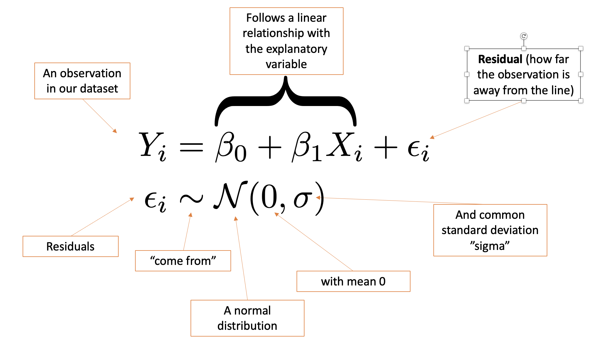
Residuals

\[ \begin{align} \text{Residual} = \epsilon_i &= \text{Observation - Predicted Value} \\ &= Y_i - (\beta_0 + \beta_1X_i) \end{align} \]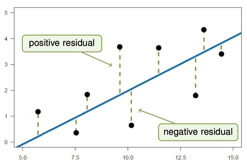

Visualizing the SLR Model

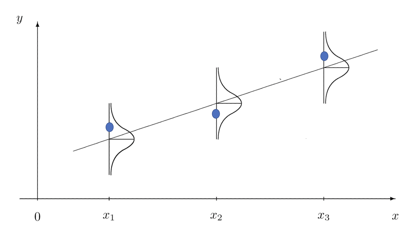
• \(\sigma\) is the standard deviation and controls the spread of the dots about the regression line. The bigger the \(\sigma\), the farther the dots from the line.

Interpreting the SLR Model

Slight change in interpretation:

• Intercept (\(\beta_0\)): If \(X=0\), we expect \(Y\) to be \(\beta_0\).
• Slope (\(\beta_0\)): If \(X\) goes up by 1, we expect \(Y\) to go up by \(\beta_1\).

Assumptions of the SLR Model

Easy way to remember what we are assuming about the population in a simple linear regression model:

• L - Linear relationship between \(x\) and \(y\)
• I - Independence (one obs. doesn’t impact the other)
• N - Normal residuals (distance from line is normal)
• E - Equal spread of residuals around the line

More on why these assumptions are important and how to check these in the next subunit.

Parameter Estimation

Parameters we want to estimate: \(\beta_0\) & \(\beta_1\) (which defines the line) and \(\sigma\) (so we know how spread out things are)

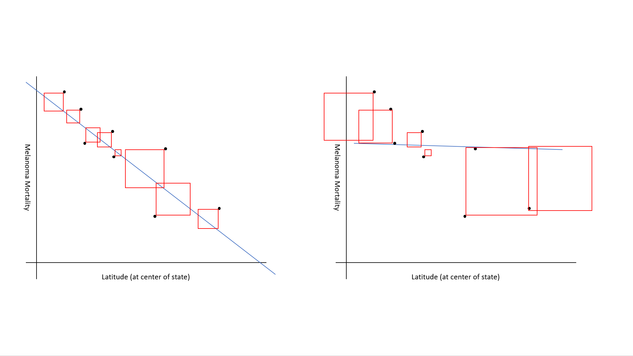
Goal: Find the line that goes “closest” to the data points.

Parameter Estimation

What do we mean by “line closest to points”? We want to find \(\hat{\beta}_0\) and \(\hat{\beta}_1\) so that: \[ \sum_{i=1}^n (Y_i - (\hat{\beta}_0+\hat{\beta}_1X_i))^2 \] is as small as possible. This is called the least squares regression line.

A few notes:

1. We “square” distances so that, for example, a 5 “above” and 5 “below” the line are the same “distance”.
2. We sum squared residuals because we look at all the data.
3. We use “hats” to denote estimates from sample (for example, \(\hat{\beta}_1\) is our estimate of \(\beta_1\))

Parameter Estimation

Parameter Estimation

How do we find \(\hat{\beta}_0\) and \(\hat{\beta}_1\) that minimizes \[ \sum_{i=1}^n (Y_i - (\hat{\beta}_0+\hat{\beta}_1X_i))^2? \]

1. Guess and check
2. Use calculus

• In either case, we’ll let the computer do the hard work for us

The Fitted SLR Model

Fitted Regression Line Equation: \[ \hat{y} = 35.653 + 0.503\times x \] where:

• \(\hat{y}\) is the fitted height value (the height value on the line)
• \(\hat{y} \neq y_i\) because \(y_i\) is an observed height

The Fitted SLR Model

A interesting point: The sign (postive/negative) of the correlation will always match the sign of the slope (positive/negative). Not the same number but the same sign.

Parameter Estimation

An estimate of \(\sigma\) is more complicated to explain (take more stats courses), so for purposes of this class, the computer estimates it for us.

• \(\hat{\sigma} =\) 3.776

How do we interpret \(\hat{\sigma}\)?

• On average, the actual student’s heights are about 3.776 inches away from the estimated heights.

Using the Analysis Tool

Using the Analysis Tool

Using the Analysis Tool

Using the Analysis Tool

Using the Analysis Tool

Practice 6.2 Question 4

Which of the following is the fitted regression line (i.e. the equation of the line of best fit) for the melanoma example?

1. \(\hat{y} = - 5.9776 + 389.1894 \times x_i\)
2. \(\hat{y} = 389.1894 - 5.9776\times x_i\)
3. \(\hat{y} = 389.1894 + 19.115\times x_i\)
4. \(\hat{y} = 19.115 -5.9776\times x_i\)

Practice 6.2 Question 4 Answer

Which of the following is the fitted regression line (i.e. the equation of the line of best fit) for the melanoma example?

1. \(\hat{y} = - 5.9776 + 389.1894 \times x_i\)
2. \(\hat{y} = 389.1894 - 5.9776\times x_i\)
3. \(\hat{y} = 389.1894 + 19.115\times x_i\)
4. \(\hat{y} = 19.115 -5.9776\times x_i\)

Practice 6.2 Question 5

How would you interpret the estimated slope in the melanoma example?

1. As mortality increases by 1, the latitude is expected to decrease by 5.9776.
2. As latitude increases by 1, the mortality is expected to decrease by 5.9776.
3. As latitude increases by 1, the mortality will decrease by 5.9776.
4. As mortality increases by 1, the latitude is expected to increase by 389.1894.
5. As latitude increases by 1, the mortality is expected to increase by 389.1894.
6. The average distance from the observed mortality to the expected (predicted) mortality is 19.115.

Practice 6.2 Question 5 Answer

How would you interpret the estimated slope in the melanoma example?

1. As mortality increases by 1, the latitude is expected to decrease by 5.9776.
2. As latitude increases by 1, the mortality is expected to decrease by 5.9776.
3. As latitude increases by 1, the mortality will decrease by 5.9776.
4. As mortality increases by 1, the latitude is expected to increase by 389.1894.
5. As latitude increases by 1, the mortality is expected to increase by 389.1894.
6. The average distance from the observed mortality to the expected (predicted) mortality is 19.115.

Assessing Model Fit

Coming back to the student height example, we had \(\hat{\sigma} =\) 3.776 which we interpret to be the difference between the actual heights and the predicted heights. Does \(\hat{\sigma} =\) 3.776 mean that the observations are “close” to the line or not?

• It’s hard to tell just from \(\hat{\sigma}\) if this is “good” or “bad” because it depends on the problem. A better measure would be a standardized measure that can be used for all regression problems.

Assessing Model Fit

Mathematical formula: \[ R^2 = 1 - \frac{\sum_{i=1}^n (Y_i - (\hat{\beta}_0 + \hat{\beta}_1X_i))^2}{\sum_{i=1}^n (Y_i - \bar{y})^2} = 0.12802 \]

Intuition:

• Formal interpretation: The percent of variability in \(Y\) that is explained by \(X\).
• \(R^2\) is between 0 and 1 with 1 meaning the data perfectly follow a line and 0 meaning the data don’t follow the line at all.
• Intuition: you can think of \(R^2\) as a “grade” for your regression line where \(R^2 = 1\) is a perfect line and \(R^2 = 0\) is a terrible line.

Using the Analysis Tool

Practice 6.2 Question 6

What is the correct interpretation of \(R^2 = 0.6798\) in the Melanoma example?

1. As latitude increases by 1, mortality increases by 0.6798 on average.
2. If latitude is zero (on the equator), mortality is expected to be 0.6798.
3. Observed mortality is about 0.6798 away from the expected (predicted) mortality.
4. About 67.98% of the variation in mortality is explained by latitude.
5. About 67.98% of the variation in latitude is explained by mortality

Practice 6.2 Question 6 Answer

What is the correct interpretation of \(R^2 = 0.6798\) in the Melanoma example?

1. As latitude increases by 1, mortality increases by 0.6798 on average.
2. If latitude is zero (on the equator), mortality is expected to be 0.6798.
3. Observed mortality is about 0.6798 away from the expected (predicted) mortality.
4. About 67.98% of the variation in mortality is explained by latitude.
5. About 67.98% of the variation in latitude is explained by mortality

Additional SLR Practice

Does a higher GPA lead to better pay? Use a the salary data and a simple linear regression model to answer the following questions:

1. What is the estimated pay for someone who completely fails college (0.0 GPA)?
2. For two people who differ by 1.0 GPA, how much higher (or lower) should the pay be for person with the higher GPA on average?
3. On average, how far away are pay amounts from estimated pay amounts?
4. How well does the GPA explain pay?

Additional SLR Practice Answers

Does a higher GPA lead to better pay? Use a simple linear regression model (and the course app) to answer the following questions (Salary dataset):

1. What is the estimated pay for someone who completely fails college (0.0 GPA)?
   • \(\hat{\beta}_0 = 51135.68\)
2. For two people who differ by 1.0 GPA, how much higher (or lower) should the pay be for person with the higher GPA on average?
   • \(\hat{\beta}_1 = 6510.04\)
3. On average, how far away are pay amounts from estimated pay amounts?
   • \(\hat{\sigma} = 10353.03\)
4. How well does the GPA explain pay?
   • \(R^2 = 0.1147\)

Key Terminology

• Least squares
• Simple linear regression model
• Slope
• Intercept

• \(R^2\)
• Relationship between correlation and slope
• Spread about regression line (\(\sigma\))